In this post we will tackle Artificial Intelligence with baby steps and try to build a very simple neural net in Java.
What is a Neural net?
A neural net is a software representation of how the brain works. Unfortunately, we do not know as of yet how exactly does the brain really work but we do know a little bit of the biology behind this process: the human brain consists of 100 billion cells called neurons, connected together by synapses. If sufficient synapses connected to a neuron fire, then that neuron will also fire. This process is known as "thinking".
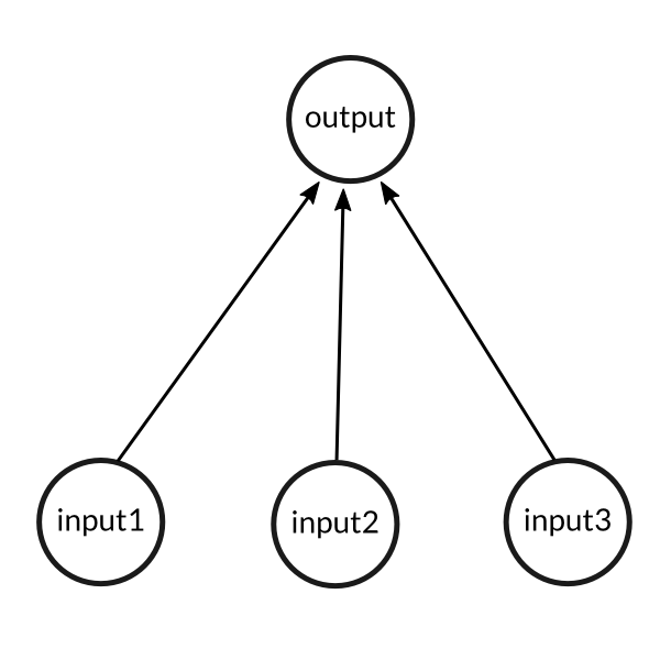
We thus try and model the above process using a very simple example that has 3 inputs (synapses) and results in a
single output (1 neuron firing).
A simple problem
We will train our above neural net to solve the following problem. Can you figure out the pattern and guess what the value of the new input should be? 0 or 1?
| Examples | Input | Output | ||
|---|---|---|---|---|
| Example 1 | 0 | 0 | 1 | 0 |
| Example 2 | 1 | 1 | 1 | 1 |
| Example 3 | 1 | 0 | 1 | 1 |
| Example 4 | 0 | 1 | 1 | 0 |
| New situation | 1 | 1 | 0 | ? |
The answer is actually very simply the value of the left-most column, i.e. 1!
The training process
So now that we have the model of a human brain, we will try and get our neural net to learn what the pattern is given the training set. We will first assign each input a random number to produce an output.
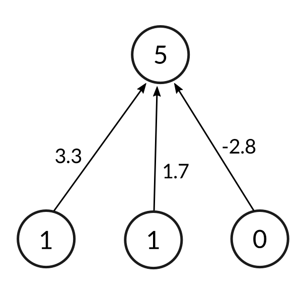
The formula for calculating the output is given as follows:
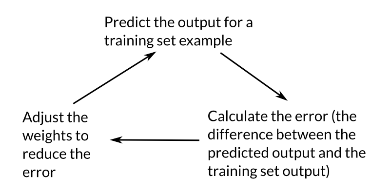
As it turns out we would like to normalize this output value to something between 0 and 1 so that the prediction makes sense. After normalization we compare the output with the expected output of our inputs. This gives us the error, or how far off is our prediction. We can then use this error to slightly adjust the weights of our neural net and try our luck on the same input again. This can be summarized in the following image:
We repeat this training process for all the inputs 10,000 times to reach a satisfactorily trained neural net. We can then use this neural net to make predictions on new inputs!
Before we jump into the implementation however, we still need to clarify how we achieved the normalization and the weight adjustment based on the error (also known as back-propagation).
Normalization
In a biologically inspired neural network, the output of a neuron is usually an abstraction representing the rate of action potential firing in the cell. In its simplest form, this is binary value, i.e., either the neuron is firing or not. Hence, the need for normalization of this output value.
To achieve this normalization we apply what is known as an activation function to the output of the neuron. If we take the example of a really simple Heaviside step function which assigns a 0 to any negative value and a 1 to any positive value, then a large number of neurons would be required to achieve the required granularity of slowly adjusting the weights to reach an acceptable consensus of the training set.
As we will see in the next section on back-propagation, this concept of slowly adjusting the weights can be represented mathematically as the slope of the activation function. In biological terms, it can be thought of as the increase in firing rate that occurs as input current increases. If we were to use a linear function instead of the Heaviside function, then we would find that the resulting network would have an unstable convergence because neuron inputs along favored paths would tend to increase without bound, as a linear function is not normalizable.
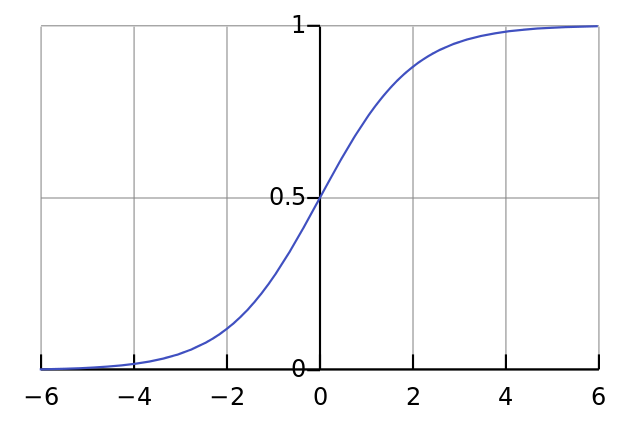
All problems mentioned above can be handled by using a normalizable sigmoid activation function. One realistic model stays at zero until input current is received, at which point the firing frequency increases quickly at first, but gradually approaches an asymptote at 100% firing rate. Mathematically, this looks like:
If plotted on a graph, the Sigmoid function draws an S shaped curve:
Thus, the final formula for the output of a neuron now becomes
There are other normalization functions that we can use but the sigmoid has the advantage of being fairly simple and also having a simple derivative which will be useful when we look at the back propagation below.
Back-propagation
During the training cycle, we adjusted the weights depending on the error. To do this, we can use the "Error weighted derivative" formula
The reason we use this formula is that firstly, we want to make the adjustment proportional to the size of the error. Secondly, we multiply by the input, which is either a 0 or a 1. If the input is 0, the weight isn't adjusted. Finally, we multiply by the gradient of the Sigmoid curve (or the derivative).
The reason that we use the gradient is because we are trying to minimize the loss. Specifically, we do this by a gradient descent method. It basically means that from our current point in the parameter space (determined by the complete set of current weights), we want to go in a direction which will decrease the loss function. Visualize standing on a hillside and walking down the direction where the slope is steepest. The gradient descent method as applied to our neural net is illustrated as follows:
- If the output of the neuron is a large positive or negative number, it signifies the neuron was quite confident one way or another.
- From the sigmoid plot, we can see that at large numbers the Sigmoid curve has a shallow gradient.
- Thus, if the neuron is confident that the existing weight is correct, it doesn't want to adjust it very much and multiplying by the gradient of the sigmoid curve achieves this.
The derivative of the sigmoid function is given by the following formula Substituting this back into the adjustment formula gives us
Code
An important but subtle point that was missed out when explaining the mathematics above was that for each training iteration, the mathematical operations are done on the entire training set at the same time. Thus, we will make use of matrices to store the set of input vectors, the weights and the expected outputs.
You can grab the entire project source here: https://github.com/wheresvic/neuralnet. For the sake of learning, we implemented all the math ourselves using only the standard java Math functions :)
We will begin with the NeuronLayer class which is just a placeholder for the weights in our neural net
implementation. We provide it with the number of inputs per neuron and the number of neurons which it can use to
build a table of the weights. In our current example, this is very simply the last output neuron which has the 3
input neurons.
public class NeuronLayer {

    public final Function<Double, Double> activationFunction, activationFunctionDerivative;

    double[][] weights;

    public NeuronLayer(int numberOfNeurons, int numberOfInputsPerNeuron) {
        weights = new double[numberOfInputsPerNeuron][numberOfNeurons];

        for (int i = 0; i < numberOfInputsPerNeuron; ++i) {
            for (int j = 0; j < numberOfNeurons; ++j) {
                weights[i][j] = (2 * Math.random()) - 1; // shift the range from 0-1 to -1 to 1
            }
        }

        activationFunction = NNMath::sigmoid;
        activationFunctionDerivative = NNMath::sigmoidDerivative;
    }

    public void adjustWeights(double[][] adjustment) {
        this.weights = NNMath.matrixAdd(weights, adjustment);
    }
}
Our neural net class is where all the action happens. It takes as a constructor the NeuronLayer and has
2 main functions:
think: calculates the outputs of a given input settrain: runs the training loopnumberOfTrainingIterationstimes (usually a high number like 10,000). Note that the training itself involves calculating the output and then adjusting the weights accordingly
public class NeuralNetSimple {

    private final NeuronLayer layer1;
    private double[][] outputLayer1;

    public NeuralNetSimple(NeuronLayer layer1) {
        this.layer1 = layer1;
    }

    public void think(double[][] inputs) {
        outputLayer1 = apply(matrixMultiply(inputs, layer1.weights), layer1.activationFunction);
    }

    public void train(double[][] inputs, double[][] outputs, int numberOfTrainingIterations) {
        for (int i = 0; i < numberOfTrainingIterations; ++i) {

            // pass the training set through the network
            think(inputs);

            // adjust weights by error * input * output * (1 - output)

            double[][] errorLayer1 = matrixSubtract(outputs, outputLayer1);
            double[][] deltaLayer1 = scalarMultiply(errorLayer1, apply(outputLayer1, layer1.activationFunctionDerivative));

            // Calculate how much to adjust the weights by
            // Since we're dealing with matrices, we handle the division by multiplying the delta output sum with the inputs' transpose!

            double[][] adjustmentLayer1 = matrixMultiply(matrixTranspose(inputs), deltaLayer1);

            // adjust the weights
            this.layer1.adjustWeights(adjustmentLayer1);
        }
    }

    public double[][] getOutput() {
        return outputLayer1;
    }
}
Finally we have our main method where we setup our training data, train our net and ask it to make predictions on test data
public class LearnFirstColumnSimple {

    public static void main(String args[]) {

        // create hidden layer that has 1 neuron and 3 inputs
        NeuronLayer layer1 = new NeuronLayer(1, 3);

        NeuralNetSimple net = new NeuralNetSimple(layer1);

        // train the net
        double[][] inputs = new double[][]{
                {0, 0, 1},
                {1, 1, 1},
                {1, 0, 1},
                {0, 1, 1}
        };

        double[][] outputs = new double[][]{
                {0},
                {1},
                {1},
                {0}
        };

        System.out.println("Training the neural net...");
        net.train(inputs, outputs, 10000);
        System.out.println("Finished training");

        System.out.println("Layer 1 weights");
        System.out.println(layer1);

        // calculate the predictions on unknown data

        // 1, 0, 0
        predict(new double[][]{{1, 0, 0}}, net);

        // 0, 1, 0
        predict(new double[][]{{0, 1, 0}}, net);

        // 1, 1, 0
        predict(new double[][]{{1, 1, 0}}, net);
    }

    public static void predict(double[][] testInput, NeuralNetSimple net) {
        net.think(testInput);

        // then
        System.out.println("Prediction on data "
                + testInput[0][0] + " "
                + testInput[0][1] + " "
                + testInput[0][2] + " -> "
                + net.getOutput()[0][0] + ", expected -> " + testInput[0][0]);
    }
}
Running our above example we see that our net has done a pretty good job of predicting when the leftmost input is 1 but can't seem to get the 0 quite right! This is because the second and third input weights both needed to have been closer to 0.
Training the neural net...
Finished training
Layer 1 weights
[[9.672988220005456 ]
[-0.2089781536334558 ]
[-4.628957430141331 ]
]

Prediction on data 1.0 0.0 0.0 -> 0.9999370425325528, expected -> 1.0
Prediction on data 0.0 1.0 0.0 -> 0.4479447696095623, expected -> 0.0
Prediction on data 1.0 1.0 0.0 -> 0.9999224112145153, expected -> 1.0
In the next post we will see if adding another layer to our neural network can help in improving the predictions ;)
References
- Tutorial by Milo Spencer-Harper on how to create a simple neural net in python.
- Tutorial by Steven Miller on building a simple neural net.
- Wikipedia article on Activation functions